39 change data labels in excel chart

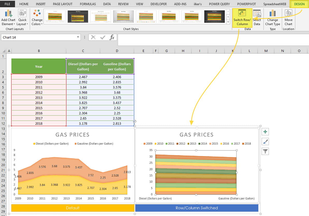
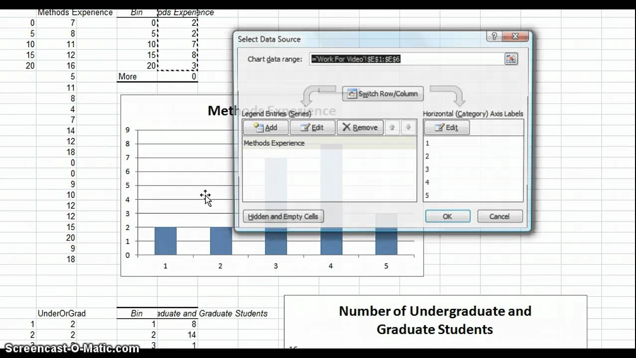
How to: Display and Format Data Labels - DevExpress When data changes, information in the data labels is updated automatically. If required, you can also display custom information in a label. Select the action you wish to perform. Add Data Labels to the Chart. Specify the Position of Data Labels. Apply Number Format to Data Labels. Create a Custom Label Entry. Change the Order of Data Series of a Chart in Excel - Excel Unlocked We can change this order. Right click on this chart and click on the Select Data option. After that select 2019 from the data series and click on the down arrow. This will move the data series 2019 below 2020. Click OK. As a result, you would see a change of order in your column chart as follows. This brings us to the end of the blog.

Excel: How to Create a Bubble Chart with Labels - Statology Step 3: Add Labels. To add labels to the bubble chart, click anywhere on the chart and then click the green plus "+" sign in the top right corner. Then click the arrow next to Data Labels and then click More Options in the dropdown menu: In the panel that appears on the right side of the screen, check the box next to Value From Cells within ...

Change data labels in excel chart

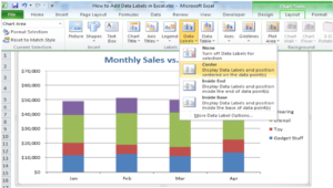
How to Add Labels to Scatterplot Points in Excel - Statology Step 3: Add Labels to Points Next, click anywhere on the chart until a green plus (+) sign appears in the top right corner. Then click Data Labels, then click More Options… In the Format Data Labels window that appears on the right of the screen, uncheck the box next to Y Value and check the box next to Value From Cells. How to Create a Run Chart in Excel (2021 Guide) | 2 Free Templates Go to the Insert tab. Click " Insert Line or Area Chart .". Choose " Line .". You now have your simple run chart as a result: Step 3. Spruce Up Your Run Chart. Technically, you're good to go, but if you're looking to improve your chart from boring to beautiful in mere moments, here's how you can quickly spruce it up. DataLabel object (Excel) | Microsoft Docs The following example turns on the data label for the second point in series one on the chart sheet named Chart1, and sets the data label text to Saturday. VB With Charts ("chart1") With .SeriesCollection (1).Points (2) .HasDataLabel = True .DataLabel.Text = "Saturday" End With End With

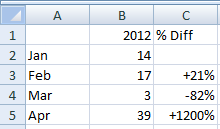
Change data labels in excel chart. Data label in the graph not showing percentage option. only value ... You need helper columns but you don't need another chart. Add columns with percentage and use "Values from cells" option to add it as data labels labels percent.xlsx 23 KB 0 Likes Reply Dipil replied to Sergei Baklan Sep 11 2021 08:47 AM @Sergei Baklan Thanks. It's a tedious process if I have to add helper columns. Modifying Axis Scale Labels (Microsoft Excel) Follow these steps: Create your chart as you normally would. Double-click the axis you want to scale. You should see the Format Axis dialog box. (If double-clicking doesn't work, right-click the axis and choose Format Axis from the resulting Context menu.) Make sure the Number tab is displayed. (See Figure 1.) Figure 1. How to Change the Y Axis in Excel - Alphr Bring the cursor to the chart where you want to change the axes' appearance. Go to "Design," then go to "Add Chart Element" and "Axes." You'll have two options: "Primary Horizontal" will... Change the Font Size, Color, and Style of an Excel Form Control Label For example, if I were to change G2 to a black color and a smaller font, the label would not show these new changes (however, it would change its text if I changed the value in G2 to something else). So to change the Label's formatting — even when it's linked to the same cell — you'll need to click the label, click the formula bar ...

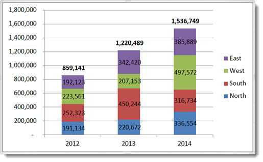
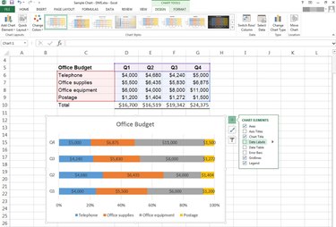
How To Add a Target Line in Excel (Using Two Different Methods) Also, click on the boxes next to the "Series names in first row" and "Categories (x labels) in the first column." Then press the "OK" button. 7. Select the change series chart type. After performing the previous actions, Excel creates a bar chart with your new data series. Right-click the new series and select the "Change series chart type" option. How to Show Percentages in Stacked Column Chart in Excel? Implementation: Follow the below steps to show percentages in stacked column chart In Excel: Step 2: Select the entire data table. Step 3: To create a column chart in excel for your data table. Go to "Insert" >> "Column or Bar Chart" >> Select Stacked Column Chart. Step 4: Add Data labels to the chart. Goto "Chart Design" >> "Add ... How can I get data labels to show for each column in a bar chart? Turn on 'Overflow text' under Data label' Format tab. Also, you can adjust the position of the Data Label by switching to 'Outside End' or 'Inside Center' so that your Data Label gets displayed properly. If this post helps, then mark it as 'Accept as Solution ' so that it could help others. Regards, Sanket Bhagwat. How to Create a Dynamic Chart Title in Excel Steps to Create Dynamic Chart Title in Excel Converting a normal chart title into a dynamic one is simple. But before that, you need a cell which you can link with the title. Here are the steps: Select chart title in your chart. Go to the formula bar and type =. Select the cell which you want to link with chart title. Hit enter.

Chart.ApplyDataLabels method (Excel) | Microsoft Docs Syntax expression. ApplyDataLabels ( Type, LegendKey, AutoText, HasLeaderLines, ShowSeriesName, ShowCategoryName, ShowValue, ShowPercentage, ShowBubbleSize, Separator) expression A variable that represents a Chart object. Parameters Example This example applies category labels to series one on Chart1. VB Copy Charts ("Chart1").SeriesCollection (1). How to Create a Waterfall Chart in Excel - SpreadsheetDaddy By default, most charts will have some form of data label automatically applied, but you can also add your own custom labels if needed. Let's see how to do it! 1. Click on your chart. 2. Navigate to the Design tab. 3. Choose Add Chart Element. 4. Click Data Labels. 5. Pie of Pie Chart in Excel - Inserting, Customizing, Formatting Inserting a Pie of Pie Chart. Let us say we have the sales of different items of a bakery. Below is the data:-. To insert a Pie of Pie chart:-. Select the data range A1:B7. Enter in the Insert Tab. Select the Pie button, in the charts group. Select Pie of Pie chart in the 2D chart section. How to Create and Customize a Waterfall Chart in Microsoft Excel Then, use the Fill & Line, Effects, and Size & Properties tabs to do things like add a border, apply a shadow, or scale the chart. Select the chart and use the buttons on the right (Excel on Windows) to adjust Chart Elements like labels and the legend, or Chart Styles to pick a theme or color scheme. Select the chart and go to the Chart Design tab.

How to Show Percentages in Stacked Bar and Column Charts in Excel

How to Find, Highlight, and Label a Data Point in Excel Scatter Plot? By default, the data labels are the y-coordinates. Step 3: Right-click on any of the data labels. A drop-down appears. Click on the Format Data Labels… option. Step 4: Format Data Labels dialogue box appears. Under the Label Options, check the box Value from Cells . Step 5: Data Label Range dialogue-box appears.

How to Make Charts and Graphs in Excel | Smartsheet

Custom Chart Data Labels In Excel With Formulas Follow the steps below to create the custom data labels. Select the chart label you want to change. In the formula-bar hit = (equals), select the cell reference containing your chart label's data. In this case, the first label is in cell E2. Finally, repeat for all your chart laebls.

Chart Data Labels in PowerPoint 2011 for Mac

Bubble Chart in Excel chart or Excel Pivot Chart I have added data labels to both dummy series in chart 3; the default Y values appear in the labels, which are aligned directly on top of the bubbles. Select the X-axis, change the minimum value to 0, and change the axis label position to No Labels. Repeat for the Y-axis, and you'll have chart 4. Select the X-axis labels, press Ctrl+1 to format ...

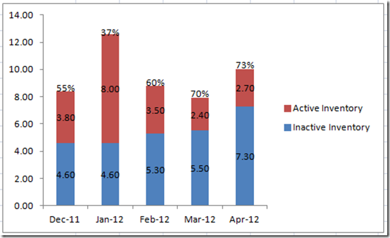
How-to Put Percentage Labels on Top of a Stacked Column Chart - Excel Dashboard Templates

How to avoid data label in excel line chart overlap ... - Stack Overflow However, it seems like the data labels will overlap with either the green dot/red dot/line. If I adjust the position of the data labels, it will only work for this 2 series of values. Sometime the values will change and cause the purple line to be above the black line, and then the data labels overlap with something else again. My question:

30 What Is Data Label In Excel - Labels Design Ideas 2020

Excel: How To Convert Data Into A Chart/Graph - Rowan University 7: To add axis titles, data labels, legend, trendline, and more, click the graph you just created. A new tab titled "Chart design" should appear. In the upper menu of that tab, you should see a section called "add chart element." 8: In "add chart element," you can customize your graph to your liking . STEP 9: Don't forget to save your work!

Charts in Excel - EASY Excel Tutorial

How to Print Labels from Excel - Lifewire Select Mailings > Write & Insert Fields > Update Labels . Once you have the Excel spreadsheet and the Word document set up, you can merge the information and print your labels. Click Finish & Merge in the Finish group on the Mailings tab. Click Edit Individual Documents to preview how your printed labels will appear. Select All > OK .

How to add or move data labels in Excel chart?

Need to change data label while hovering on dot of scatter plot in excel Post a small Excel sheet (not a picture) showing realistic & representative sample data WITHOUT confidential information (10-20 rows, not thousands...) and some manually calculated results. For a new thread (1st post), scroll to Manage Attachments, otherwise scroll down to GO ADVANCED, click, and then scroll down to MANAGE ATTACHMENTS and click ...

Area Chart in Excel

How to Create and Customize a Treemap Chart in Microsoft Excel Select the data for the chart and head to the Insert tab. Click the "Hierarchy" drop-down arrow and select "Treemap." The chart will immediately display in your spreadsheet. And you can see how the rectangles are grouped within their categories along with how the sizes are determined.

How to Use Excel to Make a Percentage Bar Graph | Techwalla

How to Change the X-Axis in Excel - Alphr Right-click the X-axis in the chart you want to change. That will allow you to edit the X-axis specifically. Then, click on Select Data. Select Edit right below the Horizontal Axis Labels tab....

34 What Is A Data Label In Excel - Labels Niche Ideas

DataLabel object (Excel) | Microsoft Docs The following example turns on the data label for the second point in series one on the chart sheet named Chart1, and sets the data label text to Saturday. VB With Charts ("chart1") With .SeriesCollection (1).Points (2) .HasDataLabel = True .DataLabel.Text = "Saturday" End With End With

How to Add Data Labels in Excel - Excelchat | Excelchat

How to Create a Run Chart in Excel (2021 Guide) | 2 Free Templates Go to the Insert tab. Click " Insert Line or Area Chart .". Choose " Line .". You now have your simple run chart as a result: Step 3. Spruce Up Your Run Chart. Technically, you're good to go, but if you're looking to improve your chart from boring to beautiful in mere moments, here's how you can quickly spruce it up.